
BLOG
Coupling ITASCA’s MPoint and FLAC Software
October 2, 2026
By David DeGagne
Bridging Large-Strain Finite Volume Mechanics and Post-Failure Runout Analysis
In our last blog, we explored how the Material Point Method (MPM) fundamentally reshapes how geotechnical engineers can simulate post-failure dynamics. By replacing meshes that conform to the material geometry with Lagrangian material points moving through an Eulerian computational grid, MPoint effectively eliminates mesh distortion while enabling seamless tracking of extreme material movement.
However, a challenge with geotechnical engineering simulation is that failure can span two distinct regimes:
- Pre-Failure and Onset (small to moderate strain): Characterized by intricate initial stress states, dynamic boundary conditions, staged construction, drainage, consolidation, ground support, and subtle constitutive behavior prior to failure.
- Post-Failure and Run-Out (extreme strain and flow): Characterized by localized shear failure leading to mass mobilization, fluidization, rapid run-out, structural impact, and final runout geometry (e.g., landslides, liquefaction, tailings dam failures).
Traditional mesh-based Finite Volume Method (FVM) solvers like FLAC excel at modeling small-to-moderate strains, offering faster run times, robust modeling tools, and easy handling of complex boundary conditions. In contrast, MPoint seamlessly simulates both small and large-strain regimes without mesh distortion issues.
But what if engineers didn’t have to choose between mesh-based models and a mesh-free post-failure simulator? What if a single framework could capture both regimes seamlessly? With ITASCA Software, you don’t have to choose. By optionally coupling MPoint with FLAC (of the same dimension and version), hybrid MPM-FVM models can seamlessly provide the best of both worlds.
Leveraging ITASCA’s experience coupling FLAC and PFC (our Discrete Element Method code), MPoint coupled with FLAC offers considerable value to engineers.
Simplify Model Building Using FLAC (zones) as Scaffolding
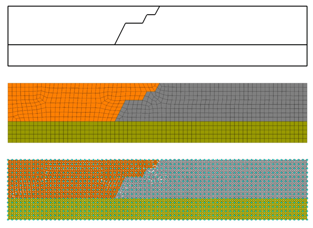
Use the same workflow that you use to build your FLAC3D or FLAC2D model mesh (e.g., Sketch tool, Griddle-Rhino3D, geometries, primitives). Using a single command, convert all, or some, zones into material points at the start or at any construction stage (Figure 1). By default, two material points per zone edge are generated and the zones are nulled. Groups, properties, and results (e.g., pore pressure, stresses, displacements, plastic state) are automatically transferred from the zones to the equivalent material points.
Accuracy and Improved Model Performance
A single finite volume zone solves much faster than multiple material points. To balance accuracy and efficiency, material points are restricted to regions undergoing large deformations, such as active shear band failures and run-out zones. Far-field behavior is represented using zones, which significantly speeds up simulations. Modeling performance can be further optimized using Adaptive Material Conversion logic where the model initially consists entirely of zones, which can be automatically converted into material points only where and when needed, based on the detection of poor zone conditions (e.g., zone quality < 0.4), as shown in Figure 2.

Figure 3 compares the solve performance of MPoint3D alone (blue) against coupled MPoint3D–FLAC3D (red) for the simple slope example, evaluated over 8,000 steps at three resolution levels (0.25 m, 0.5 m, and 1.0 m). All benchmarks were run on a 12th Gen Intel Core i9-12900HK laptop (64 GB RAM).
The results show a linear relationship between material point count and solve time. Crucially, the coupled model achieves a 5–10x speedup over the standalone MPoint3D model. This efficiency gain occurs because only 10–15% of the zones—specifically those experiencing localized large strains—convert into material points.

Complex Boundary Conditions
One of the greatest challenges in purely MPM simulations is handling dynamic boundary conditions during seismic events (e.g., earthquake ground motions). Standalone MPM grids struggle to accurately apply non-reflecting (quiet) boundaries or energy-absorbing formulations (free-field) because material points continuously change positions relative to grid boundaries. Coupling FLAC continuum zones with MPoint solves this fundamental challenge.
By surrounding active material points with an outer buffer of FLAC zones, simulations can leverage FLAC’s native quiet and free-field boundary conditions during dynamic seismic analysis. The quiet boundaries absorb outgoing body waves via viscous dashpots to prevent artificial wave entrapment and energy buildup within the domain. Simultaneously, the free-field boundaries run parallel 1D continuum models along the lateral edges to match infinite free-field motion, preventing rigid-box distortions as seismic energy propagates upward. (Note: Dynamic analysis requires the Dynamic Option.)
As illustrated in Figure 4, by coupling FLAC free-field zones at the far edges with MPoint in the central failure/run-out region, engineers can apply real time-history earthquake acceleration records at the base while ensuring mathematically rigorous seismic wave propagation throughout the entire domain.

A Common Framework
Rather than running two separate software programs connected by some external data exchange, ITASCA incorporates MPoint and FLAC natively within a single, shared computational environment called the Common Framework. Working with either (or both) is simple and straightforward, although a valid license for each is required. Simply set up a FLAC model, and only a few additional MPoint commands are needed to instantly or adaptably convert some or all zones into material points.
Because both methods share ITASCA’s extensive Constitutive Model Library (e.g., Mohr-Coulomb, Modified Cam-Clay, NorSand, CySoil), state variables mapped from a FLAC zone into an MPoint particle retain their stress history and yield parameters without needing complex material mapping. FLAC-supported user-defined models (C++ UDM) can also be utilized with a minor modification of its C++ file.
With zone conversion, MPoint coupled with FLAC allows engineers to model the entire life cycle of a slope or earthwork structure, providing an efficient and integrated solution that bridges small-strain continuum analysis and post-failure large-strain flow within a single unified UI/UX experience.
If you know FLAC3D or FLAC2D, you already know MPoint.
How Does Coupling Work?
Instead of running two separate models and exchanging forces across a complex boundary interface, FLAC zone gridpoints and MPoint material points can be treated in the same way. Where FLAC material meets MPoint material, hybrid points are created using existing FLAC gridpoints that are also treated like material points by MPoint, forming a type of glue between the two methods. Zone gridpoint forces on hybrid points are applied to the material point background grid, and hybrid point velocity is set from the MPM grid-to-point mapping. Hybrid points maintain kinematic continuity where FLAC zones transition into MPoint particles. This ensures stress waves and displacements travel seamlessly across the boundary without generating artificial stiffening, gaps, or energy dissipation.
To optimize performance, material points within FLAC zones are created dynamically when a zone condition threshold is breached (e.g., zone quality < 0.4) over a specified radius. At this point, any poor-quality zone(s) are deleted, and material points are created in their place to maintain large-strain runout, while stable regions continue using the more computationally efficient FLAC zones. Hybrid points function as an adaptive buffer during this shift, interpolating stress tensors, pore pressure, and density to maintain continuum stress state integrity.
Figure 5 illustrates this dynamic capability through a zero-damping dynamic analysis of a cantilever beam under gravity load. Here, four structural combinations of zones and material points are evaluated showing plots of vertical displacement contours alongside tip y-displacement histories across several full deflection cycles, displaying millimeter accuracy.
Figure 6 shows a cone penetrometer simulation comparing coupled zone-material points (left) to material points only (right). Initially, the coupled model consists of only zones, with a small region of material points, to help initiate penetration near the tip of the cone penetrometer (represented using PFC2D-type walls) that were above the ground surface to begin with. Zones can be distinguished from material points as black outlined regions.

Figure 6 shows a cone penetrometer simulation comparing coupled zone-material points (left) to material points only (right). Initially, the coupled model consists of only zones, with a small region of material points, to help initiate penetration near the tip of the cone penetrometer (represented using PFC2D-type walls) that were above the ground surface to begin with. Zones can be distinguished from material points as black outlined regions.

A First in Geotechnical Analysis
To model geotechnics effectively, engineers need tools that balance speed, precision, and the ability to handle extreme movement. This is where coupling FLAC and MPoint comes in—combining the strengths of grid-based finite volume modeling with MPoint-based simulation.
Efficiency: Running a purely material particle model across a large domain is computationally expensive. Coupling keeps the bulk of the stable model domain in more efficient FLAC zones while reserving MPoint calculations only for regions undergoing severe distortion or runout. Run time improvements for coupled models can be 5–10x faster than an MPoint-only model, depending on the simulation.
Accuracy: Standard FLAC can suffer from zone meshing issues when material flows or collapses. Coupling passes the failing material to MPoint before mesh distortion halts the calculation and allows engineers to model the entire life cycle of a slope or earthwork structure without the need to transfer information between different solution codes.
Ease of Use: MPoint shares the same common framework as other ITASCA software and, as a continuum method, uses the familiar workflow of FLAC and its breadth of constitutive models. Coupling MPoint and FLAC is simple, allowing zones to be converted to material points at any point based on poor zone quality in regions undergoing high deformations. Groups, displacements, stresses, extra variables, and more are automatically transferred between zones and material points. And finally, coupling an inner core of material points to an exterior group of zones makes application of dynamic boundary conditions trivial.
MPoint marks a major milestone: it provides a dedicated, commercially supported MPM environment tailored specifically for geotechnical engineering practice. Integrated within ITASCA’s familiar and trusted framework, MPoint brings powerful, yet practical, large-deformation modeling into day-to-day workflow. While MPoint provides standalone capabilities for large-strain post-failure modeling, its real power multiplies when MPoint is coupled with FLAC to seamlessly transition from zones to material points within a single, unified analysis workflow to simplify model building, maximize modeling performance, and include advanced boundary conditions for dynamic analyses.
MPoint is now available with the release of ITASCA Software v9.8. Existing FLAC2D and FLAC3D users can start modeling complex run-out analyses with coupled FLAC-MPoint simulations by purchasing an MPoint license.
Join us for an in-depth look at MPoint in our webinar “Modeling Large Deformation with MPoint” on October 7, 2026 at the time that works best for you:
Author

Dave DeGagne
Senior Engineer, Technical Marketing